Blog

  • Mevo+ vs. Square Omni Head to Head Accuracy Comparison

    I was briefly in possession of both units and did a head to head comparison outdoors. I am also a lefty for those that think the Omni is unreliable for left-handed players.
    In summary:

    • Both units obtained shot shape and ball data that qualitatively agreed with the shot shapes I saw in real life
    • They share unanimous and close agreement on ball speed, ball direction, and most launch characteristics
    • For club data on irons, they shared excellent agreement on face and path data
    • For club data with driver, they disagreed significantly on face and path data, and I am inclined to think the Mevo+ was more accurate
    • Without a Trackman or GCQuad there is no gold standard for comparison, so “accuracy” in the title may be a misnomer and “agreement” more appropriate, but I found everything to be very close to expectations other than driver face/path data on the Omni

    I think there are two ways to look at these — the shot-to-shot differences, as well as the differences when averages are compared to smooth out the noise.
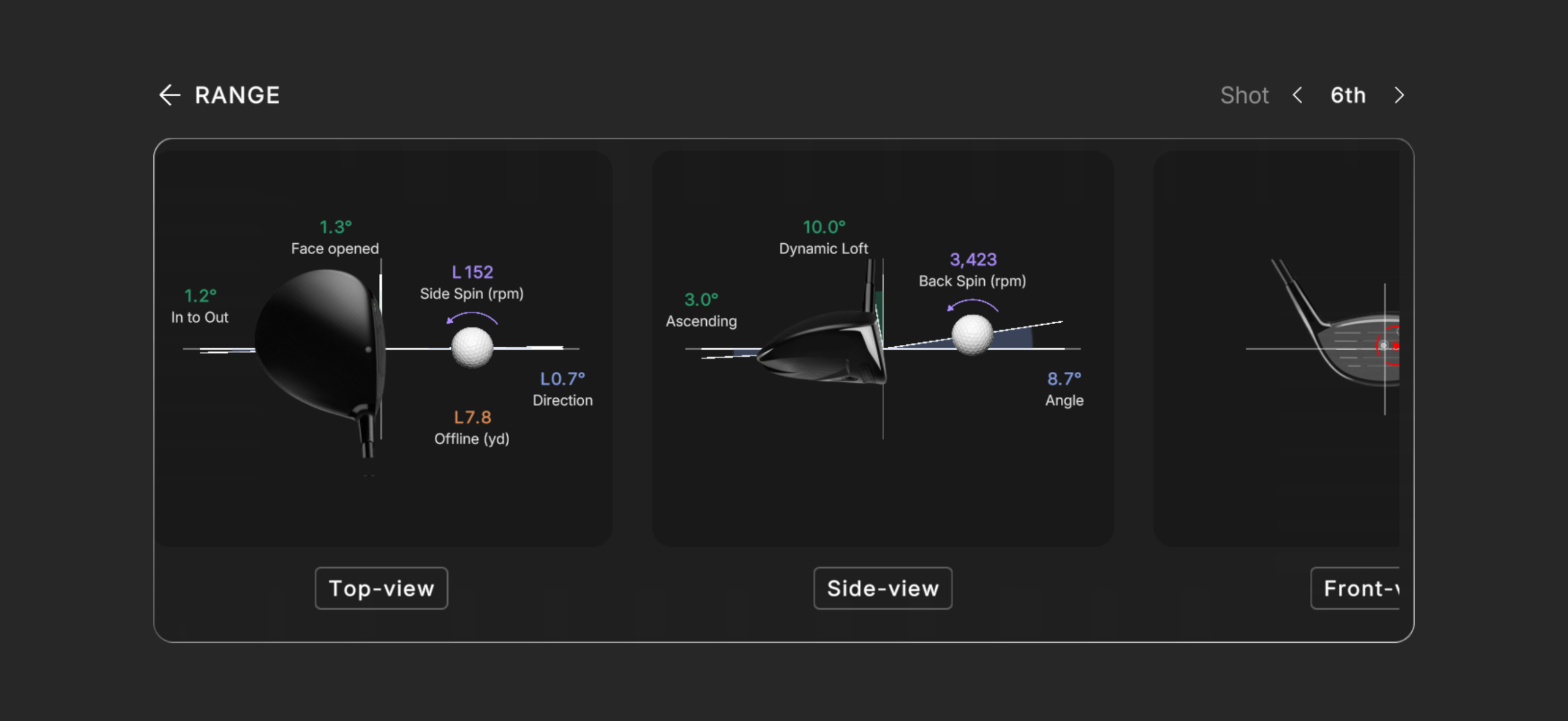
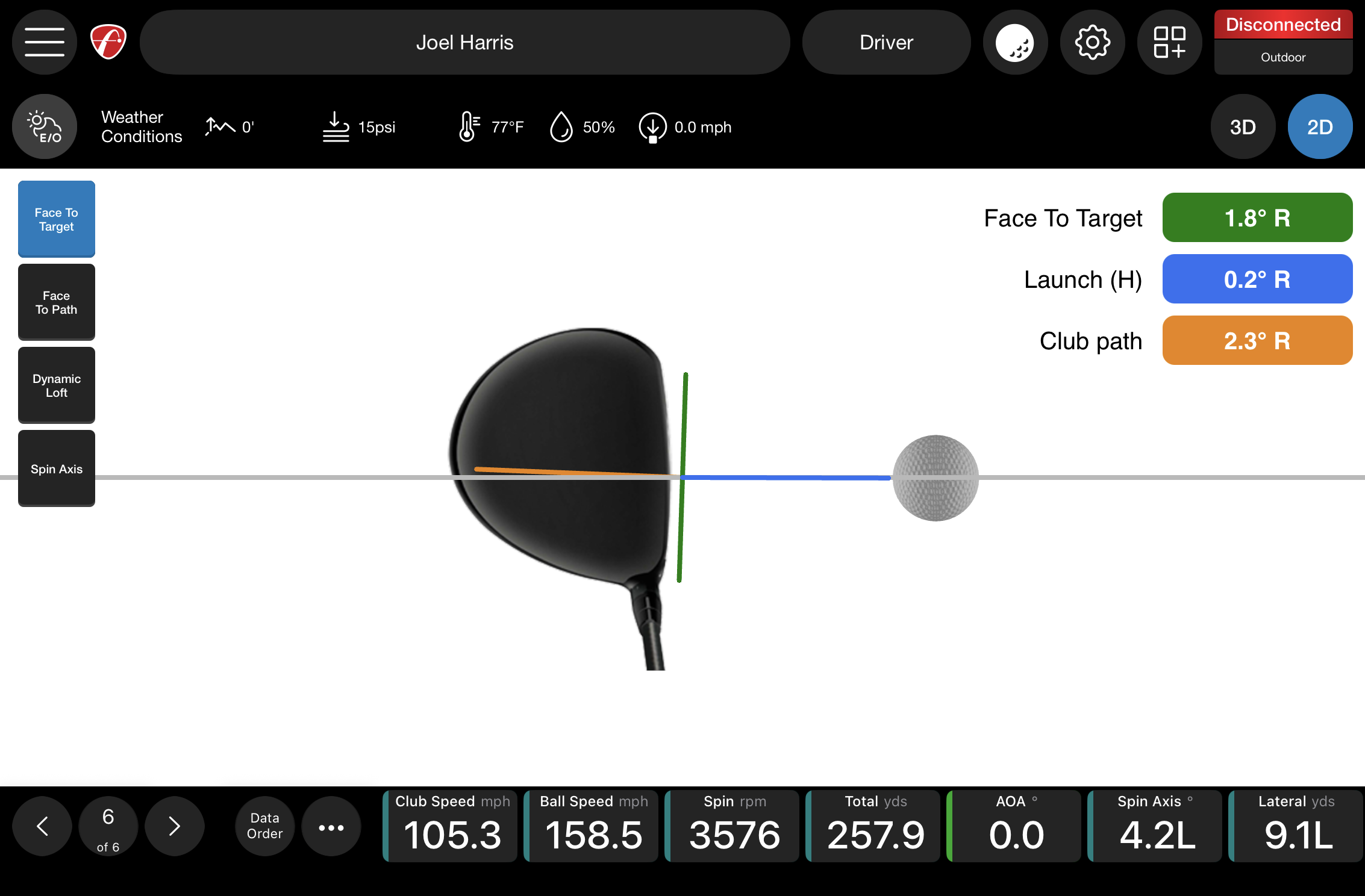
    Averaged club data:

    The most notable finding in all of this was that the Mevo+ and Square Omni share excellent agreement for irons, but disagreed significantly on woods. As a lefty, I play a cut with my driver and accordingly am used to 2-3 degrees RIGHT for club path, with a face angle somewhere between square to the path or slightly left to path (i.e., 0-2 degrees LEFT to target). The Mevo+ was within what I expected with club path 2.2R with a face to path slightly left of that. The Square Omni felt my path was relatively square with a slightly open face. Ultimately this would also make a fade, so it has not made up false physics for these shots, but it arrived at that conclusion in a different way.

    ClubMevo pathSquare pathMevo faceSquare faceNotes
    Mini driver2.2 R1.9 L2.6 R3.0 RPath disagreement!!!
    8 iron2.6 L4.1 L1.9 L1.5 LGood
    Driver2.2 R0.01.6 R0.7 LEverything disagreement!!!
    4 iron1.9 L1.8 L0.7 L0.9 LExcellent
    7 iron3.3 L3.1 L1.1 L1.1 LExcellent

    Averaged data (7 iron):

    MeasurementNMevo+ meanSquare mean
    Ball Speed11118.02 mph116.82 mph
    Club Speed987.89 mph84.68 mph
    Launch Direction111.32 L1.52 L
    Launch Angle1114.06°14.30°
    Carry11164.16 yd163.04 yd
    Spin116,221 rpm6,496 rpm
    Dynamic Loft1121.29°20.33°
    Club Path113.29 L3.13 L
    Face Angle111.10 L1.06 L
    Attack Angle11-7.31°-3.78°

    Averaged data (Driver):

    MeasurementNMevo+ meanSquare mean
    Ball Speed13152.90 mph151.64 mph
    Club Speed11102.04 mph103.41 mph
    Launch Direction130.35 L0.68 L
    Launch Angle139.62°9.68°
    Carry13245.55 yd240.07 yd
    Spin133,016 rpm3,362 rpm
    Dynamic Loft1311.02°11.37°
    Club Path132.22 R0.02 L
    Face Angle131.60 R0.73 L
    Attack Angle130.46°1.15°

    Shot to shot correlation with 7 iron:

    MeasurementNMevo+ vs Square r
    Ball Speed110.987
    Club Speed90.474
    Launch Direction110.810
    Launch Angle110.974
    Carry110.872
    Spin110.513
    Dynamic Loft110.930
    Club Path110.456
    Face Angle11−0.015
    Attack Angle110.214

    Shot to shot correlation with driver:

    MeasurementNMevo+ vs Square r
    Ball Speed130.968
    Club Speed110.785
    Launch Direction130.963
    Launch Angle130.992
    Carry130.862
    Spin130.478
    Dynamic Loft130.961
    Club Path130.048
    Face Angle130.729
    Attack Angle130.154

    Angle of attack had particularly poor correlation on these. The Mevo+ had me at 6-9 degrees down and the Square had me at 1 to 6 degrees down. Off to the right I have pictured the raw data, but with shots where one read -8 and the other read -1, this really killed the correlation.
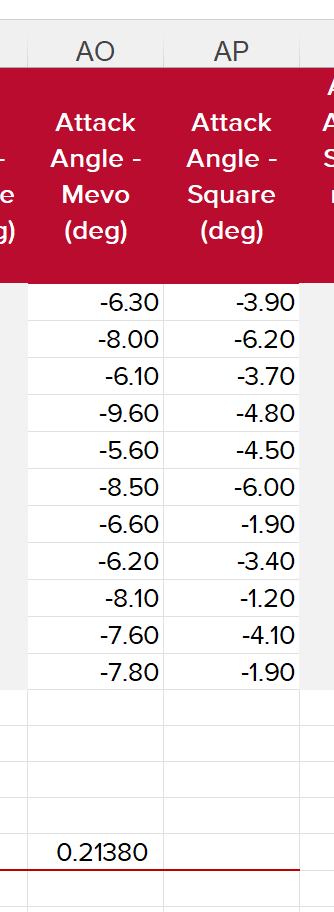
    angle of attack data and its r of 0.214

    Methods:

    Range balls were used, which run a bit spinnier and launch a bit higher on all shots besides wedges. But my goal is comparison so I don’t think it matters much. All balls were in good shape and I excluded a ball if it was well-worn with smoothed dimples which would affect the real-life aerodynamics, which is something the Mevo+ would pick up on as it is watching the actual launch and trajectory of the ball, while the Square Omni’s physics simulator / calibrated data would not.

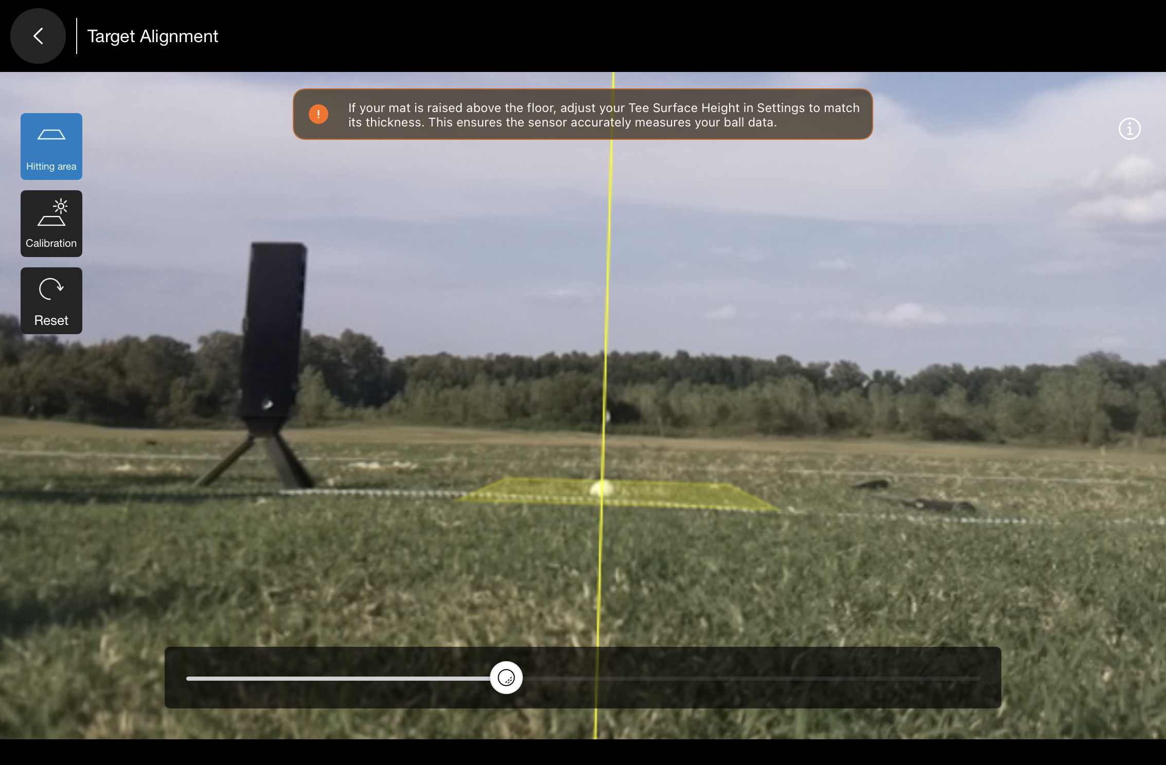
    I did my best to get a setup where the ball was in the ideal reading zone for both launch monitors.

    Excel’s CORREL function was used to get within-club r values for each club and its ball data.

    This is r, as in Pearson’s r, which measures only how well two variables move together, not whether they have the exact same values. So if the Square consistently under-reads some Mevo+ metric by 5%, but does so consistently, it can still have a perfect 1.000 correlation. So as alluded to in the first paragraph, this was more about correlation than accuracy, and all I can conclude from this is how well the readings tend to ‘move together’.

    Below is an example of how this looked for ball speed for the 5 shots hit with an 8 iron. This was repeated for every metric and every set of paired shots within each club. I used assistance from AI to do this en masse once I confirmed it was doing so correctly for several data, because it was very tedious to do it all in Excel.
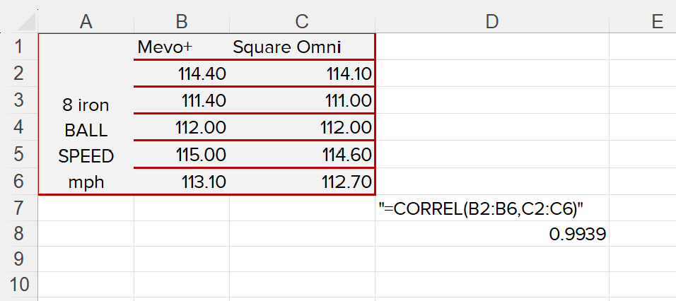
    generating correlation for the 8 iron ball speed values, as an example
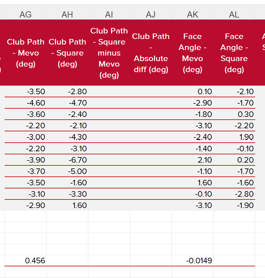
    example of the r values being generated for face and path correlation for 7 iron shots. The L/R directions were all changed to +/- for easier analysis. Much like Trackman conventions for direction, POSITIVE is RIGHT and NEGATIVE is LEFT

    Raw data for nerds:

  • Solutions to infinite square well problems and visualization of energy quantization

    Solutions to infinite square well problems and visualization of energy quantization

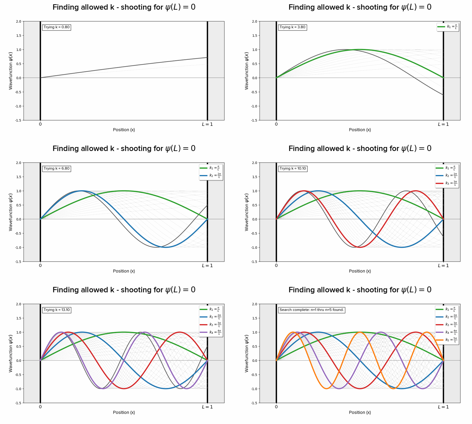
    In MIT’s OpenCourseWare Physics 8.04 course the professor poses walking through many values of k where only special values of k will satisfy the boundary conditions imposed upon us. For these problems I did not find good visualizations, and I wanted to make a good visualization of particle in a box / infinite square well problems. This is just a gif visualization of the boundary conditions in the well forcing energy quantization, and I have the assumption the reader is familiar with these infinite square well / particle in a box problems.

    An animated simulation of the shooting method used to find energy eigenfunctions for an infinite square well. The plot shows trial wavefunctions scanning through different wavenumbers (k), highlighting the first five successful solutions that satisfy the boundary condition psi(L)=0 in distinct colors
    TISE:22md2ϕdx2+V(x)ϕ=Eϕand V(x)=0 in well\text{TISE:}-\frac{\hbar^2}{2m}\frac{d^2\phi}{dx^2}+V(x)\phi=E\phi \text{; \quad and V(x)=0 in well}
    22mϕ(x)=Eϕ(x);ϕ+k2ϕ=0;k2=2mE2 -\frac{\hbar^2}{2m}\phi”(x)=E\phi(x) \quad \text{;}\quad \phi”+k^2\phi=0 \text{;}\qquad k^2=\frac{2mE}{\hbar^2}
    solutions of form ϕE(x)=Acos(kx)+Bsin(kx)\text{solutions of form }\phi_E(x)=A\cos(kx)+B\sin(kx)

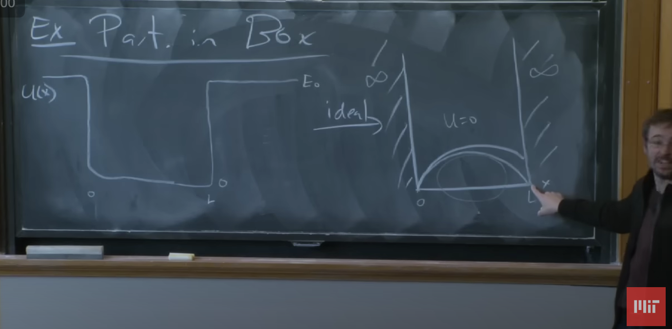
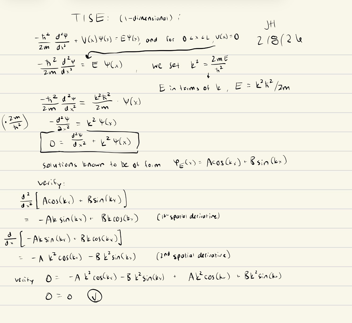
    I have my work briefly summarized on this page. Where ϕ(0) = 0 forces A to 0, leaving only the sine term to survive, he posed walking through values of k until we find those very special values of kL for which we hit 0 at position L.

    Allan Adams chalkboard lecture on particle in a box solutions. The equivalent to the Matplotlib animation above - from 8.04 lecture 6 (https://ocw.mit.edu/courses/8-04-quantum-physics-i-spring-2013/resources/lecture-6/)
    The chalkboard equivalent to the Matplotlib animation above – from 8.04 lecture 6

    I found it really cool that even in the most trivial, idealistic, simplified example of solving the TISE, we’re faced with the peculiar fact that energy [eigenvalues] are discrete and greater than zero.

    This is not an actual attempt at numerical solutions of these problems and uses a rudimentary shooting method — the Python script, which was generously written by Claude, increments through k values in steps of 0.3 (chosen so there’s about 10 steps between solutions) until it lands on a candidate solution, then switches to a bisection algorithm that picks out the solution. I am definitely not the first to do this, though I do think I am the first to clean it up nicely in a gif. There are multiple people who have treated this more robustly than I have (this Bachelor’s thesis from Austria, this guy’s YouTube video on numerical methods for this exact topic). I will probably try to follow this with a similar visualization of the simple harmonic oscillator, as those failed solutions explode (diverge) at infinity which is a much more dramatic visualization for how our energies are forced to discrete values. The math is much more complicated and I don’t know how I’m going to do that.

  • Visualizing Sports Betting with Python; Evolution of a Bankroll Over Time With +EV Betting

    The point of this article is to make the abstract concept of expected value more accessible with some nice GIFs. The mathematical and computational underpinnings of what we do here are the modeling of a stochastic process best described as a discrete-time random walk. Among many other things these have important implications in financial modeling and this lecture from a University of Leicester economics course provides a summary.

    Assumptions for below:

    • Your starting account balance is $1000
    • Your unit size is $10 (you place $10 on each bet)
    • We somehow know the true probability for the outcomes of sporting events
    • We place 500 bets

    Reality for >90% of players: Losing money in the long run (two-sided lines of -110 / -110 for an event whose true probability is 0.5)

    You are betting on an event which is truly, unambiguously, 50/50 (e.g., the coin toss at the Super Bowl) and your sportsbook offers two-sided lines of -110 / -110. In other words, as is the case with any bet, if you pick wrong you lose your entire staked amount. If you win, you profit ~90% of your stake. This is effectively what every sportsbook offers and how every casual gambler plays.

    Bankroll of 10 different players over the course of 500 bets. Do you lose money in the long run? YES!!

    The exact numbers depend very much on the sportsbook and the market you are betting on. Some markets have much more generous lines. Main lines are much more liquid than player props, and sportsbooks are much more confident in their NFL main lines than, say, Major League Table Tennis games props, and will offer better odds accordingly. The first few paragraphs on BettorOdds’ write-up describe this better than I will.

    Simulated for 10 different players, you can see the natural ebb and flow of a bankroll. There is a natural variance and some players “get hot” but in the long run, the loss of money is inevitable when the odds are -110 (i.e., your profit on winning bets is 90% of your stake). Put in more statistically sound terms — you will lose money when placing bets with negative expected value.

    I ran it over 500 iterations, much to the dismay of my laptop’s CPU. I’d love to do more but I’m at a coffee shop and my laptop is on battery. Anyway– note that almost every bettor loses money in the long run. The occasional gambler will find luck and find himself up over a short period of time — the simulation indicated by the orange line finished at a bankroll of $1002 after 500 bets. All others were down some significant amount. Despite some brief stretch of luck found by orange, over infinitely many iterations (bets), every bettor will lose money. This is the multi-billion dollar investment thesis of Las Vegas sportsbooks and we are certain it is true from practice as well as probability.

    A perfectly fair sportsbook who offers odds that perfectly reflect the true probability of events occurring

    Bankroll of 10 different players over the course of 500 bets.

    This theoretical sportsbook does not wish to make any money, but only provide liquidity to the betting market. In the long run, your return on investment will tend towards zero and averaged over many simulations, your bankroll will remain near its starting balance… well, probably. Kind of. Not really. Below I will take a quick detour on random walks in stochastic processes— I would ignore this and skip to the next image if that sounds boring.

    In reality what I describing above is an unbiased random walk, and there is a small but non-zero chance that variance wipes out your bankroll entirely. In other words, you go on an exceedingly cold streak that wipes out your bankroll entirely, and now you are broke with no possibility of recovery. It may be easier to imagine this if your account balance is $100 and your bet size is $50. Lose your first two bets and it’s over. Even if you work your way up to a $200 balance, lose 4 bets in a row and it’s over. It’s not hard to imagine a coin landing on heads 4 times in a row. If you flip the coin 10,000 times, the probability approaches 1.

    This phenomenon is described as “gambler’s ruin” and there are mathematical tools for describing the probability that you are broke after t bets, with some starting bankroll n. Or the probability that you reach a certain account balance after t bets without being ruined. A real-life gambler, if he is playing responsibly, assigns his bet size to some percent of his bankroll such that losing money in the long run won’t entirely bankrupt him but slowly tick down his bankroll closer and closer to zero with each loss.

    The mathematical underpinnings of this are beyond the scope of my knowledge but I think would be well within the reach of undergraduate probability classes. See this lecture from an MIT course on probability in computer science. There is a LibreText chapter on Introductory Probability which describes it in section 12.1.

    Sportsbook offers line of +110 for an event whose true probability is 0.5:

    Bankroll of 10 different players over the course of 500 bets.

    Sportsbook offers line of +130 for an event whose true probability is 0.5:

    Bankroll of 10 different players over the course of 500 bets.

    As you will basically never find lines this good without boosts / promos, this is effectively promo betting or promo hunting; taking a normal -110 / -110 main line and applying a 50% boost to it. Even if you randomly choose sides, hitting 50% of these bets will lead to positive returns. You have some wiggle room and do not even need to hit half of them.

    There will never be a main line or prop bet whose line strays this far from the true odds for more than a few minutes. There are computers and humans who will hammer the bet until the sportsbook either removes it or lowers its odds to minimize risk.

    How can we say we know the true probability for a sporting event?

    I hope to write this part later– I wanted to publish the graphics today

    Thanks!

    • This simulation uses the following Python libraries:
      • NumPy (https://numpy.org/): Developed and maintained by the NumPy community
      • Matplotlib (https://matplotlib.org/): Developed and maintained by the Matplotlib development team
      • Pillow (https://python-pillow.org/): Developed and maintained by the Pillow contributors.
    • Grinstead and Snell’s Introduction to Probability was helpful.
    • This lecture from a University of Leicester economics course was helpful.