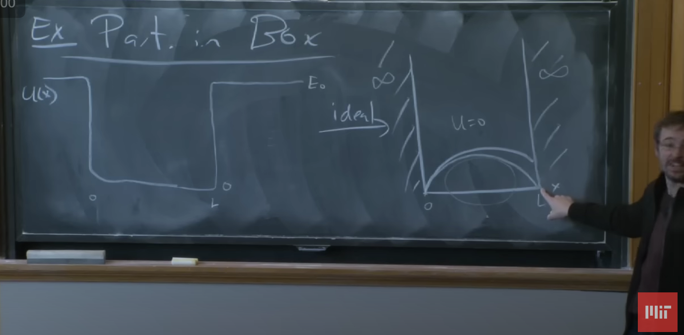
Solutions to infinite square well problems and visualization of energy quantization

In MIT’s OpenCourseWare Physics 8.04 course the professor poses walking through many values of k where only special values of k will satisfy the boundary conditions imposed upon us. For these problems I did not find good visualizations, and I wanted to make a good visualization of particle in a box / infinite square well problems. This is just a gif visualization of the boundary conditions in the well forcing energy quantization, and I have the assumption the reader is familiar with these infinite square well / particle in a box problems.

An animated simulation of the shooting method used to find energy eigenfunctions for an infinite square well. The plot shows trial wavefunctions scanning through different wavenumbers (k), highlighting the first five successful solutions that satisfy the boundary condition psi(L)=0 in distinct colors

\text{TISE:}-\frac{\hbar^2}{2m}\frac{d^2\phi}{dx^2}+V(x)\phi=E\phi \text{; \quad and V(x)=0 in well}

-\frac{\hbar^2}{2m}\phi”(x)=E\phi(x) \quad \text{;}\quad \phi”+k^2\phi=0 \text{;}\qquad k^2=\frac{2mE}{\hbar^2}

\text{solutions of form }\phi_E(x)=A\cos(kx)+B\sin(kx)

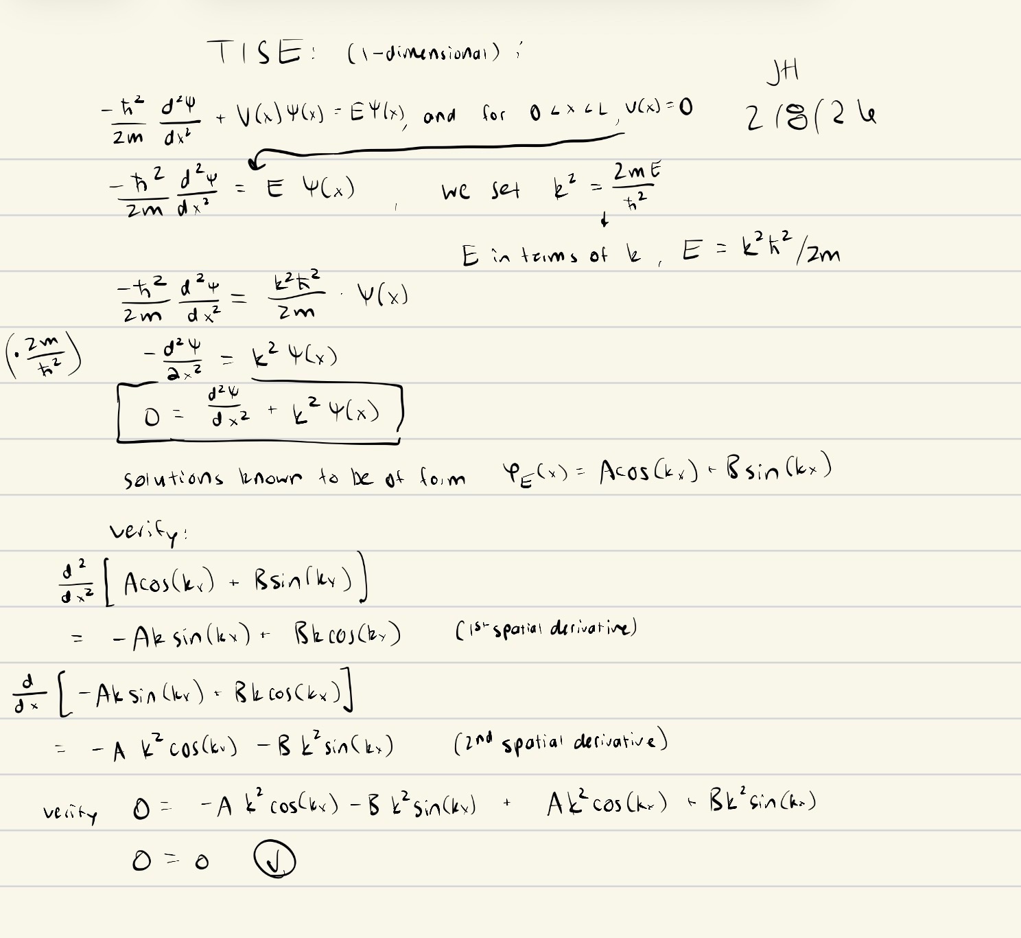
I have my work briefly summarized on this page. Where ϕ(0) = 0 forces A to 0, leaving only the sine term to survive, he posed walking through values of k until we find those very special values of kL for which we hit 0 at position L.

Allan Adams chalkboard lecture on particle in a box solutions. The equivalent to the Matplotlib animation above - from 8.04 lecture 6 (https://ocw.mit.edu/courses/8-04-quantum-physics-i-spring-2013/resources/lecture-6/) — The chalkboard equivalent to the Matplotlib animation above – from 8.04 lecture 6 (https://ocw.mit.edu/courses/8-04-quantum-physics-i-spring-2013/resources/lecture-6/)

I found it really cool that even in the most trivial, idealistic, simplified example of solving the TISE, we’re faced with the peculiar fact that energy [eigenvalues] are discrete and greater than zero.

This is not an actual attempt at numerical solutions of these problems and uses a rudimentary shooting method — the Python script increments through k values in steps of 0.3 (chosen so there’s about 10 steps between solutions) until it lands on a candidate solution, then switches to a bisection algorithm that I most certainly didn’t write myself. I am definitely not the first to do this, though I do think I am the first to clean it up nicely in a gif. There are multiple people who have treated this more robustly than I have (this Bachelor’s thesis from Austria, this guy’s YouTube video on numerical methods for this exact topic). I will probably try to follow this with a similar visualization of the simple harmonic oscillator, as those failed solutions explode (diverge) at infinity which is a much more dramatic visualization for how our energies are forced to discrete values. The math is much more complicated and I don’t know how I’m going to do that.

Solutions to infinite square well problems and visualization of energy quantization

Comments